Eco Notepad

Where is euro area inflation in relation to the “Phillips cone”?

Published on 26 July 2019
Authors : Clémence Berson, Hadrien Camatte, Antoine Lalliard, Julien Le Roux

Post n°125. The “Phillips cone” is a range of possible values for inflation obtained using different specifications of the Phillips curve. The Eurosystem’s June 2019 projection for euro area inflation is slightly below the median forecast in the Phillips cone for the entire projection horizon, and even slightly below the cone at the start of the horizon. This suggests that the Eurosystem’s projection is fairly prudent.

Image Chart 1: The euro area projection is prudent relative to the Phillips cone Source: Eurostat, Eurosystem, authors’ calculations Note: after the first quarter of 2019, the black line shows the Eurosystem’s June 2019 projection.
Chart 1: The euro area projection is prudent relative to the Phillips cone Source: Eurostat, Eurosystem, authors’ calculations Note: after the first quarter of 2019, the black line shows the Eurosystem’s June 2019 projection.

The Phillips curve – a useful tool for central banks

The Phillips curve establishes a relationship between inflation and the economic environment. It was first introduced 60 years ago, but is the focus of repeated debate, notably regarding whether or not it is still relevant (see Rue de la Banque No. 56; for a review of the literature, see Le Bihan, 2009).

Inflation projections, including those compiled by the Eurosystem, are based on more complex models than the Phillips curve. However, the latter is still widely used by economists as it makes it possible to check whether a macroeconomic scenario is coherent using a reduced-form model based on a few key variables. Nonetheless, there is still some uncertainty over the “best specification” of the Phillips curve to use (ECB, (2019)), and notably over the choice of explanatory variables (see Béreau, Faubert and Schmidt (2018)). These uncertainties justify using a range of specifications rather than just one. This approach, known as “thick modelling”, is the one we follow in this post.

The Phillips cone shows the relationship between prices and the economic environment

The “Phillips cone” can be defined as a range of possible values obtained using different specifications of the curve, and a central forecast corresponding to the median of the different models. For each date, the cone is determined by the gap between the highest and lowest simulations resulting from the chosen specifications.

The Phillips cone shown here is obtained using a set of three standard specifications. First we use a variable that measures the state of the economic environment (output gap, unemployment rate or the gap between the unemployment rate and the structural unemployment rate), lagged by a quarter. In a second step, we add a variable for external prices as an indicator of the strength of global demand or of external shocks (relative import prices, competitors’ import prices which correspond to the export prices of the euro area’s main trading partners, oil prices or the change in the price of other commodities). Last, the estimation is enhanced with a lagged expression of HICP inflation (harmonised index of consumer prices) to reflect the stickiness of price formation and of agents’ inflation expectations. In some equations, we also add a variable corresponding to variations in VAT to take into account changes in tax policy (see Figure 1).
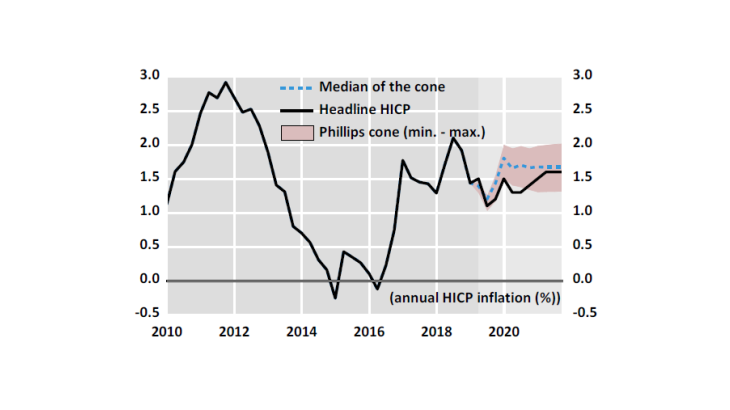
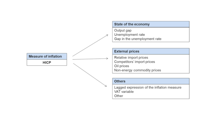
Image Figure 1: Specifications of the Phillips cone using three categories of variable
Figure 1: Specifications of the Phillips cone using three categories of variable

Different readings depending on the Phillips specification used

The forecast may be interpreted differently depending on the Phillips curve specification used.

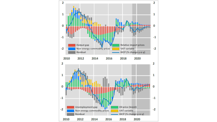
In the first example (Chart 2), we use a Phillips curve that includes the output gap and relative import prices. Import prices and sluggish euro area activity weighed to a similar extent on inflation between 2013 and 2016. In 2018, import prices made a positive contribution to inflation, while the negative output gap stopped dragging on prices. Over the forecast horizon, and assuming oil prices remain almost stable, import price growth is expected to slow. The contribution of import prices to inflation, in terms of its deviation from the average, is projected to decline, becoming almost nil. The euro area output gap is also expected to be close to zero and should no longer drag on inflation. At the end of the horizon, the residuals are seen making a negative contribution, and inflation only comes back towards its long-term average in 2021.

In another example (Chart 2), we simulate a Phillips curve using the gap in the unemployment rate and the current and lagged oil price. This time, the activity variable makes a stronger contribution to the pick-up in inflation versus its long-term average. In this specification, the residuals are markedly less negative and, at the end of the horizon (end-2021), inflation is slightly above its long-term average, unlike in the previous case.

Image Chart 2: Varying impacts of activity and import prices on the inflation forecast Source: Eurostat, Eurosystem’s projections, authors’ calculations Note: percentage point deviation from the sample average
Chart 2: Varying impacts of activity and import prices on the inflation forecast Source: Eurostat, Eurosystem’s projections, authors’ calculations Note: percentage point deviation from the sample average

Comparison with the Eurosystem’s inflation projection

We compare the Eurosystem’s inflation projection for the euro area, published in June 2019, with the forecasts obtained using the Phillips cone and the median of the Phillips curves. According to the Eurosystem’s June 2019 projection, euro area HICP inflation is expected to be 1.3% in 2019, 1.4% in 2020 and 1.6% in 2021. The figures are below the median value of the cone for 2019, but within the cone in 2020 and 2021, and in line with the median at the end of the horizon (see Chart 1). This suggests that the Eurosystem’s scenario for the trajectory of inflation is somewhat prudent.

Nonetheless, the recent weakness in euro area inflation readings (1.4% year-on-year in the second quarter of 2019) is hard to explain using the Phillips curve. The prolonged presence of negative residuals in several specifications shows the limits of this type of reduced-form model. Even so, the Phillips curve is still a useful element in the central banker’s toolkit for analysing inflation and checking whether the Eurosystem’s projection scenario is coherent.